Let’s recall a fundamental interpretation of probability, known as the “frequentist” interpretation. If I say that the probability of getting heads on the flip of a coin is 50%, what I am really saying is that any experiment done with this coin should result in half of the tosses landing as heads. In other words, the frequency of a head turning up is half of the total tosses.
This should be contrasted with the “Bayesian” interpretation, which says that prior to the first flip, we expect the half; however, as the experiment continues, we should be updating our “priors” with the new information. In this way, our expectation of future experiments (using the same coin) is updated, so that if the coin is in fact unfair, our worldview updates in order to account for this fact.
In finance, we encounter real-world probabilities all the time. For instance, you can access the Chicago Mercantile Exchange (CME) website to view the real world probability that the Fed will hike interest rates in the coming meetings. Analogously, the Society of Actuaries has an Economic Scenario Generator Excel workbook that can produce possible future outcomes of various economic indicators, including various interest rates, aggregate returns and volatilities, various credit spreads, etc.

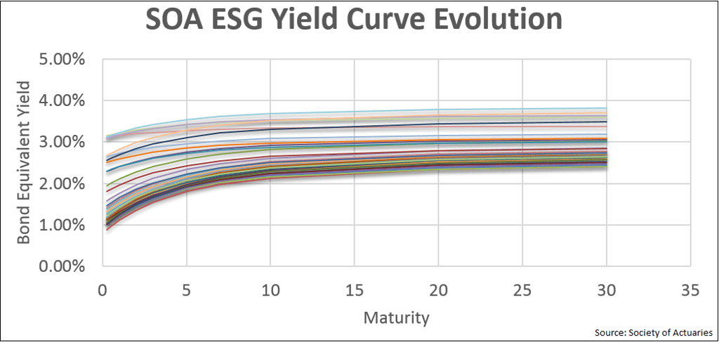
The outcomes are treated as equally likely, and the probability distribution is recovered in the frequentist way, in that the more likely outcomes have more results “clustered,” as we see in the above graph. Above, there are many clustered around the current yield curve shape and very few with higher rates and flattened curves. The probability distributions involved are determined through econometric modeling, which is a hybrid of the statistical time series analysis that captures historical analysis (and assumes what is likely to occur is what happened in similar circumstances in the past) and economic principals, such as three principal components driving the entire yield curve.
Many have probably heard of “risk neutral” probabilities, which Merton taught us play a central role in the dynamic replication of equity options in the Black-Scholes-Merton framework. This probability measure is determined from market expectations and ensures that any instrument that can be statically hedged will be priced exactly, and that the probabilities of movements are taken from option prices. These two pieces of information—together with a model for equity movements—exactly specify the prices of all other tradeable securities. The resulting probability measure is known as the risk-neutral measure, as it makes market participants indifferent on buying or selling the derivative security.
Complications
Many factors complicate this picture, such as transaction costs and asymmetric borrowing and lending rates; however, the Black-Scholes-Merton model has stood the test of time for derivative pricing. One reason this is true is that, while no one believes that stocks movements are lognormally distributed, the Black-Scholes implied volatility gives us a way to perform relative value analysis. For instance, if an option is trading at a price of 20, and another at a price of 3, which is relatively “richer”? The question is unanswerable unless you know all of the other factors: strike, underlying price, and time until maturity. That being said, given two implied vols, say 20% and 25%, you can immediately make the assessment that the 25% volatility is “richer,” as option prices are monotonically increasing in the volatility input.
All probability measures are associated with something called a “numeraire,” which is a fancy word for how you measure relative wealth. Other measures are also used in derivative pricing. The two major ones are Risk-neutral measure and T-forward measure.
The former is associated with using wealth relative to a bank account accruing at the risk-free rate. The latter is associated with measuring wealth with respect to a zero coupon bond that matures at the same time as the derivative payoff. You can now see that the numeraire is highly tied to how one discounts future cash flows.
When using ESG to project future economic scenarios, all derivatives must be priced within those scenarios using the risk-neutral measure consistent with that scenario. When this requires a Monte Carlo pricing for exotic derivatives or variable annuities, this is known as stochastic on stochastic.
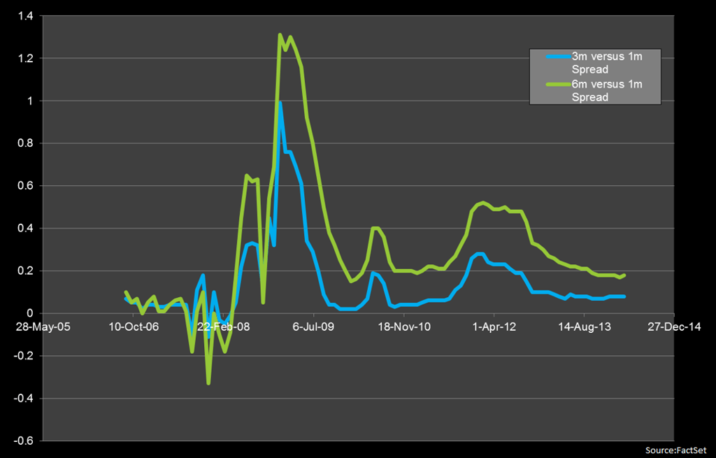
As an aside, the role of discounting drastically changed in 2008 as a result of the global financial crisis. Prior to 2008, there was a single LIBOR yield curve that could be used to both project LIBOR rates and for discounting. LIBOR basis swap instruments existed; however, their market quotes (measured in basis points which, when added to the shorter tenor leg, result in a par swap). If the usual compounding relationship of LIBORs hold, these swaps should be priced with very small, which was typically seen prior to 2008.

However, as can be seen in the above graph, after 2008, the spreads became persistently non-zero. The usual compounding relationship no longer held, implying that a single curve is no longer capable of projecting all tenors of LIBORs, which was implicitly required when using a single curve.
The biggest repercussion of this was that there was no longer an “obvious” curve to use for discounting, which begs the question. After much deliberation in the industry, two answers rose to the fore:
- Theoretical: John Hull, Professor of Derivatives and Risk Management at the Rotman School of Management at the University of Toronto, said that the answer was in quantitative finance, a fundamental principal of derivative pricing is to use the risk-free curve for discounting, as opposed to, say, a corporate finance project funded at the company WACC, with potentially a spread due to the riskiness of the project. Hull argued that the best proxy for the risk free rate is the overnight index swap average rate.
- Practical: Traders argued that they have to pass on the funding cost to the market, and therefore the funding rate should be used to discount the swaps. For fully collateralized swaps, the funding rate is precisely the collateral rate, which all contractually specify the rate to be the overnight index swap average rate.
Therefore, at least for fully collateralized swaps, the two answers agree. Currently, all swap market data must be priced using OIS discounting, and both the LCH and the CME use OIS discounting to value their swaps. This elevated the market of OIS swaps, and it is now a central curve for all economies that have a liquidly traded swap market.
| Economy |
Overnight curve |
| USD |
Fed Funds |
| EUR |
EONIA |
| GBP |
SONIA |
| JPY |
TONAR |
| CAD |
CORRA |
As alluded to earlier, it is well known that a set of stock options can be used to imply the risk-neutral probabilities of stock movements. This distribution will be peaked around the forward price of the stock, which is necessary so that the equity forwards in the market are exactly priced. It was a long held belief that option prices were silent on real world probabilities; however, recently Stephen Ross, Professor of Financial Economics at the MIT Sloan School of Management, found a surprising result that these same option prices can be used to determine the real world probabilities, and therefore the market expected real world drift of the equity! This was met with skepticism in the quantitative finance community, until Peter Carr, Chair of the Finance and Risk Engineering Department at NYU Tandon School of Engineering, re-derived the results using modern pricing theory. In the paper, he echoes the initial shock and disbelief:
“Those of us raised on the Black-Merton-Scholes paradigm find Ross’s claims to be startling. If one can value options without knowledge of expected return, then how can one use option prices to infer expected return? On the other hand, if expected returns are increasing in volatility, then higher option prices imply higher volatility and higher expected return,” Carr wrote in Risk, Return, and Ross Recovery.
Carr hinted at exactly why this might be the case: that according to standard portfolio management theory, there is a relationship between risk and return. The higher the risk, the higher the expected return. Since volatility is the standard measure of portfolio risk, and volatility is exactly the quantity implied by option prices, there should be no surprise that a connection between the two is possible.
An open question is whether or not this can be leveraged by investors to obtain alpha. One study by Audrino, Huitema, and Ludwig in 2014 found that a trading strategy based on the Ross recovery theorem outperformed the S&P 500 by 8.1%.
