Earlier this year, reports began to emerge indicating that 2016 was the first year since the end of European sovereign debt crisis in which fund flows into passive investment vehicles exceeded that into actively managed products. While this is certainly the case for European investors, similar trends now seem to be appearing in U.S. markets as well.
Whether this heralds the start of another salvo in the active vs. passive debate remains to be seen, but it provides a backdrop to explore these trends.
In our last article, we argued that while Brinson-Fachler attribution has its advantages, each iteration only captures a portfolio manager’s skill in respect to a single factor. We now look to address that issue, by introducing a multi-factor performance attribution model that decomposes excess return using a multi-factor methodology. This approach can provide portfolio managers with complementary analysis that can strengthen their case for the higher fees that active management commands, and it has the added bonus of allowing them to uncover strategies that are heavily exposed to style factors, and thereby compete with low-cost, strategic beta funds.
Risk-Based Attribution Methodology
Assuming a basic multi-factor decomposition of stock returns, we can define portfolio return as:
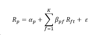
Where:
 = the portfolio’s exposure to a given risk factor
 = the return of the given risk factor at time
 = the residual (idiosyncratic) stock return
This approach provides a mechanism through which portfolio returns can be expressed as a product of the allocation to, and performance of, a series of common drivers of stock returns (factors) and individual stock level components.
The first question, when looking at this decomposition, is how we define the factors, which are deemed to drive stock returns. In each case, the choice of a multi-factor model provides a series of descriptors that decompose security- and portfolio-levels returns. More importantly, the use of a robust multi-factor risk model provides a direct connection between expected sources of portfolio risk (defined as the expected variance of absolute or relative return) and the drivers of the subsequently realized return.
Having selected an appropriate multi-factor model, the next step is to fit this within a performance attribution framework. At FactSet, we refer to this as risk-based performance attribution, which uses the chosen factor model to decompose excess return into two terms: a Factor Effect and a Stock Specific Effect.
The Factor Effect represents the product of the active exposure to a given factor and its associated return, compounded through the measurement period:

The Stock Specific Effect is a residual term, calculated as the difference between excess return (Total Effect) and the Factor Effect.
Like Brinson, risk-based performance attribution is an arithmetic model of attribution; however, as allocation decisions are accounted for within the Factor Effect, it is not subject to the same grouping bias. As a result, the portfolio level decomposition of excess return remains consistent across grouping strategies.
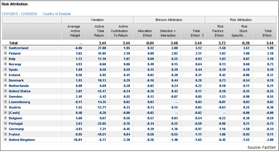
As we see above, taking account of multiple allocation decisions in the risk-based performance attribution framework tells a very different story to Brinson, which showed the manager’s outperformance coming predominantly from stock selection. In contrast, risk-based performance attribution shows our manager’s outperformance dominated by systematic tilts (372 basis points), rather than stock selection, which actually represents a drag on performance of -28 basis points. For an active manager with a focus on stock selection, running this model alongside Brinson reveals features of the portfolio hitherto unseen.
Next, we can use the model to decompose performance into the underlying sources to understand how the 372 basis points break down across factors.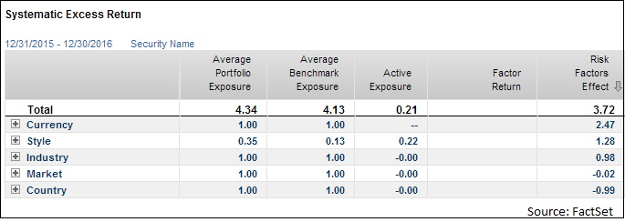
By grouping individual factors together by their respective type, we see that Currency decisions have been the largest contributor to excess return, contributing 247 basis points. Within Currency, decisions to underweight negatively performing GBP and overweight outperforming NOK have the greatest positive impact.

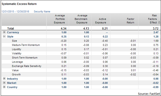
Style factors represent the second largest positive contributor to excess return at 128 basis points. Using this Axioma model, the Style block contains factors that are characterized by the fundamental attributes of a security (factors such as Value, Growth, Momentum, Liquidity, etc.). As seen below, our fund exhibits a strong tilt towards small cap securities, which appears to have been a good decision, driving the largest portion of excess return (169 basis points) from fundamental tilts.
Active Management vs. Strategic Beta
Over the last few years, these types of factors have been used increasingly as a foundation for passive investment vehicles from so-called Smart Beta products to a range of ETFs. Whether these types of strategy incorporate a fundamentally based weighting scheme or mimic the returns of factors based on fundamental characteristics, each will typically maintain a pre-defined factor tilt and come with the lower management costs associated with passive investment vehicles.
There are a number of arguments that suggest decomposition of returns within a multi-factor framework can determine whether a manager is truly active or simply banking return obtainable with a lower cost Smart Beta investment vehicle. Given the increasing focus on active vs. passive management and the costs associated with each, this type of insight becomes increasingly valuable. By using the above framework, but revising our factor structure, we can discern differences between allocation towards factors, which could be considered Smart Beta, and more active management decisions.
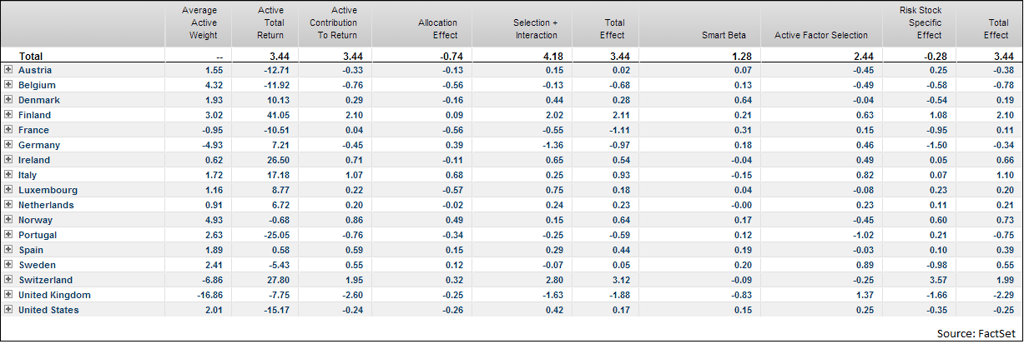
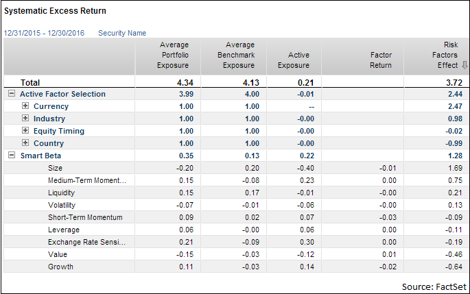
Here we introduce two new terms in place of the Factor Effect. The strategic beta component represents the portion of excess return attributable to fundamental risk factors (i.e., the return that can arguably be obtained through lower cost strategic beta investment vehicles). The Active Factor Selection represents allocation decisions across Country, Currency and Sector/Industry groups. A final group, marked above as Equity Timing within the Active Factor Selection, is comprised of an equity market factor and represents manager decisions around the expected performance and volatility of equities.
Such a framework is flexible enough to account for different fund investment styles. For example, a European Small Cap Growth fund may include both the Size and Growth factors within the Active Factor
Selection, with the remainder of the Style factors captured as unintended exposures to “Smart Beta.”
Time-Series View of Active Management
To demonstrate the manager’s skill further, we can introduce a timing element to the analysis:
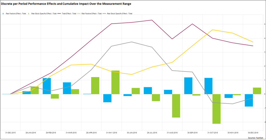
In the chart above, we break down the discrete per period performance effects (columns) and the cumulative impact over the measurement range (lines). Here we can see that the manager’s stock selection yielded positive excess return through the first half of 2016, only to be eroded between July and October.
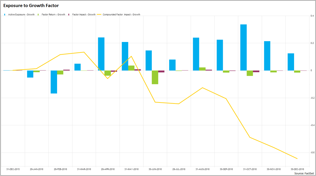
Analyzing factors in isolation helps to uncover another distinction between active management and passive tracking of a style. Looking at the Growth factor as an example, we see that our manager has initially underweighted those stocks with a high exposure to growth relative to the benchmark. This yields positive return during the first three months of the year when the factor underperforms. Our manager then increases exposure to this factor (perhaps on the expectation that growth stocks are set to rally), but after some initial success in May, fails to rebalance to account for poor performance.
As a multi-factor model of attribution, risk-based performance attribution can provide additional insight into the decisions that underpin portfolio performance. In the active management space, this affords us the ability to show the impact of multiple allocation decisions that influence stock selection as well as the strength of those convictions. From a passive standpoint, risk-based performance attribution can affirm that a product designed to track the performance of specific factor signals is able to do so consistently.
Read part one here: The Benefits of Active Management and the Shortcomings of Brinson-Fachler Attribution
